How to Add Sort Drop Down in Excel

This tutorial will demonstrate how to alphabetize a drop down list in Excel & Google Sheets.

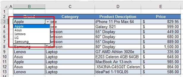
When we enter repetitive data into Excel, it can sometimes be useful to have a drop down list of options to select from. A powerful new feature of Excel 365 is the ability to sort data and only show unique data in a list due to a new feature called Dynamic Array Functions.

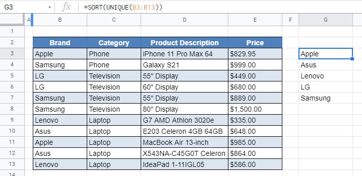
In order to obtain a drop down list of unique values sorted into alphabetical order, we need to use two of these new functions, namely the UNIQUE and SORT Functions. We can then use Data Validation to create our drop down list from the data returned by these functions.

Note that it's also possible to sort alphabetically using VBA.

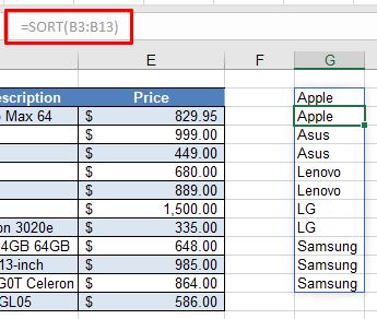
The SORT Function

The SORT Function allows us to sort a list of data into alphabetical order.

In a blank cell to the right of our data, we can type the following formula:

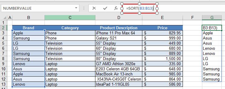
When we press ENTER, or click the check mark to enter the formula into Excel, a list of sorted values from the selected range will appear beneath the cell that we have entered our formula into. This is known as the "spill range."

The spill range automatically outputs all the unique values that are contained in the selected range. Notice that in the formula bar, the formula is greyed out in this spill range due to the fact that it is a Dynamic Array Formula. If we were to delete the formula in cell G2 for example, then the spill range would be cleared as well. The spill range is identifiable by the thin blue line that appears around it.

The UNIQUE Function

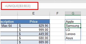
The UNIQUE Function is another Dynamic Array Function that allows us to extract unique values from a list.

In a blank cell to the right of our data, we can type the following formula:

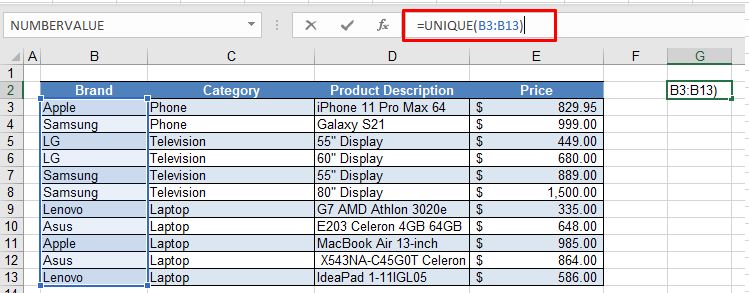
As with the SORT Function, as soon as we press the ENTER key, the UNIQUE Function will spill over to the spill range and fill in the column below the cell where we have entered the formula. The list will only show unique values from our original selected range and as it is a Dynamic Array Formula, we cannot amend or alter the formula in this spill range.

Combining the SORT and UNIQUE Functions

By combining the SORT and UNIQUE Functions together, we can obtain a list that only shows unique values and is sorted into alphabetical order.

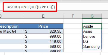
NOTE: It does not matter in which order we nest the functions; we could also use the formula =UNIQUE(SORT(B3:B13)).

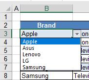
Creating the Drop Down List

We can now use this range of cells to create a drop down list to select from using Data Validation.

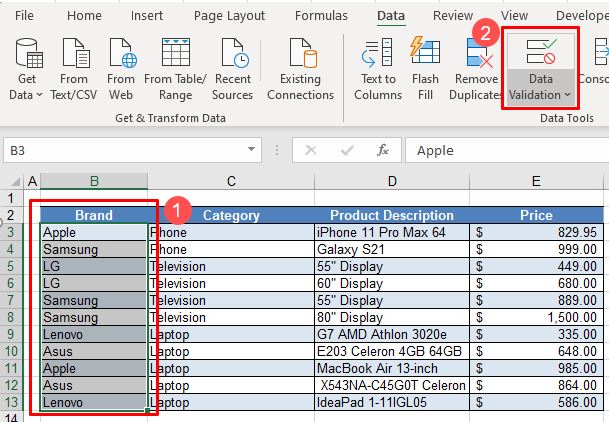
1. Select the range of cells where we wish the drop down list to appear, and then in the Ribbon, select Data > Data Validation.

2. Now select List from the Allow list, then type the formula for the Source of the list.

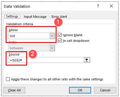
It is necessary to put the hashtag (#) after the formula to let Excel know that we require the entire spill range and not just the value in the individual cell (e.g., G2).

3. Click OK to create the sorted drop down list in the selected range.

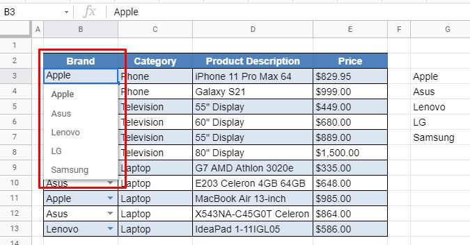
How to Alphabetize a Drop Down List in Google Sheets

The SORT and UNIQUE Functions work the same way in Google Sheets as they do in Excel.

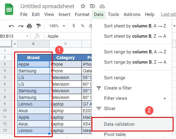
1. To create the drop down list, highlight the range of cells that will contain the drop down list, and then in the Menu, select Data validation.

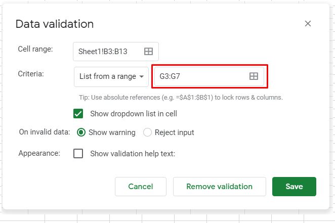
2. While the cell range to contain the drop down lists will automatically be filled in from our selection above, we need to enter the Criteria. List from a range is automatically selected and then we need to enter the entire cell range for the criteria list (e.g., G3: G7). The hashtag functionality that Excel uses does not exist in Google Sheets.

3. Click Save to insert the sorted dropdown list into the Google spreadsheet.

How to Add Sort Drop Down in Excel

Source: https://www.automateexcel.com/how-to/drop-down-sort-alphabetize/

Share this post